IWISTAO Blog is the official platform of IWISTAO HIFI MINIMART, dedicated to high-fidelity audio and DIY electronics. We focus on tube amplifiers, output and power transformers, speaker enclosures, and Bluetooth audio technologies, including HiFi Bluetooth speakers, headphones, and tube-based acoustic systems. The blog shares product insights, technical knowledge, and practical guides for audiophiles and audio builders worldwide.
LS3/5A and Tube Amplifiers: A Practical Matching Experience
Published by IWISTAO
Why LS3/5A is often described as “not happy without tubes,” and what really makes the pairing work.
1. Understanding the Nature of the LS3/5A
The BBC LS3/5A is a rare loudspeaker in the hi‑fi world. Small in size, limited in absolute output, yet extraordinarily revealing of system quality. It is not a speaker that rewards brute force or excessive power.
Whether in its 11‑ohm or 15‑ohm versions, the LS3/5A does not primarily demand current delivery. Instead, it responds most clearly to voltage stability, linearity, and micro‑dynamic resolution. Its lightweight cone and dense midrange information expose the character of the driving amplifier with little mercy.
This fundamental trait explains why amplifier choice matters more here than with many modern loudspeakers.
2. Why Tube Amplifiers Fit the LS3/5A So Naturally
Many listeners encounter similar issues when driving LS3/5A with transistor amplifiers:
Thin or dry tonal balance
Over‑tight imaging with limited harmonic bloom
Reduced emotional engagement at low listening levels
When a well‑designed tube amplifier replaces the solid‑state unit, the change is usually not subtle:
Midrange density increases noticeably
Vocals gain body, stability, and realism
Reverberation tails become longer and more natural
Music remains complete and expressive even at low volume
This is not simply “tube warmth.” It is the result of a driving method that aligns closely with the LS3/5A’s electrical and mechanical behavior.
3. 15 Ohm vs 11 Ohm: Differences from a Tube Perspective
15‑Ohm Versions
Classic 15‑ohm LS3/5A models tend to integrate exceptionally well with traditional tube output transformer designs. In practice, they offer:
Higher mid‑high frequency density
A more relaxed and unforced presentation
Greater sense of depth and room ambience
For listeners committed to tube amplification, the 15‑ohm version often feels more natural and less constrained.
11‑Ohm Versions
Later 11‑ohm LS3/5A models are more tolerant of solid‑state amplification and present a slightly more neutral, controlled character. With tube amplifiers they still perform beautifully, though often with a touch less openness and bloom compared to their 15‑ohm counterparts.
4. Tube Types and Their Sonic Tendencies
300B Single‑Ended Amplifiers
Among all options, 300B single‑ended designs often deliver the most convincing results with LS3/5A:
Exceptionally rich and textured midrange
Strong vocal intimacy and emotional presence
Stable tonal balance at very low listening levels
This pairing reflects the original design philosophy behind LS3/5A more closely than almost any other.
These tubes can sound extraordinarily transparent and refined, but demand ideal system conditions. Room acoustics, volume level, and recording quality become critical. When perfectly matched, the result is exquisite; when not, the sound may feel fragile or undernourished.
5. Output Impedance and Transformer Taps
A frequently overlooked issue is output transformer matching. Using an 8‑ohm tap to drive an 11‑ohm LS3/5A will not damage equipment, but it is rarely optimal.
Impedance mismatch affects damping factor, bass articulation, and tonal density. Whenever possible, selecting the transformer tap closest to the loudspeaker’s nominal impedance yields the most balanced and coherent sound.
6. The Overlooked Strength: Low‑Volume Listening
Perhaps the greatest advantage of the LS3/5A paired with tube amplification lies in low‑volume performance. Late‑night listening reveals:
Complete vocal structure
Stable instrumental proportion
Preserved emotional narrative
Many modern high‑resolution systems fail precisely in this area.
Conclusion
The LS3/5A is not a universal loudspeaker. It has clear limits in scale and output. Yet when driven by a carefully chosen tube amplifier and listened to within its natural boundaries, it offers something rare: a long‑term, emotionally sustainable relationship with music.
It may not always impress instantly, but it is remarkably difficult to replace.
Grounding Design for EL34 Single-Ended Tube Amplifiers
Published by IWISTAO
In real-world DIY and small-scale production experience, nearly 80% of first power-up failures in EL34 single-ended (SE) tube amplifiers are caused by incorrect grounding implementation, not by circuit topology, tube quality, or transformer selection.
This article presents an engineering-grade grounding guide for EL34 SE amplifiers, including a star-ground overview (with labeled return paths), an “incorrect vs correct” comparison, and topology-aware grounding notes for CRC vs CLC power supplies. There is a circuit diagram for EL34 SE tube amplifier below.
1. Why Grounding Is Critical in EL34 SE Amplifiers
Unlike push-pull amplifiers, a single-ended EL34 output stage provides no cancellation of power-supply ripple. Any disturbance appearing on the ground reference is directly amplified as part of the audio signal.
Cathode voltage: approximately 30–40 V
Quiescent current: approximately 60–80 mA
Because the output stage draws continuous DC current, ground conductors carry large ripple currents. Even milliohms of shared ground impedance can generate audible voltage modulation.
2. The Three Ground Domains Inside an EL34 SE Amplifier
A common conceptual error is treating “ground” as a single universal node. In practice, an EL34 SE amplifier contains three distinct ground domains:
Power ground: EL34 cathode network, output stage returns, screen returns
Rectifier / reservoir ground: rectifier return, first reservoir capacitor loop
Signal ground: RCA input return, driver stage cathodes, volume pot return, feedback reference
Correct grounding separates these domains and connects them at one—and only one—defined reference point.
3. EL34 SE Grounding Overview Diagram (Star Ground with Labeled Return Paths)
The star ground point should be located at (or immediately adjacent to) the negative terminal of the main B+ filter capacitor. All return paths converge here while remaining electrically separated along their routes.
The goal is simple: keep the high-current output-stage return and the rectifier charging pulse return from sharing impedance with the low-level signal reference. In an EL34 SE amplifier, any shared ground impedance becomes signal.
There is an example for the grounding layout of EL34 SE tube amplifier below.
4. Key Equations (Reference)
Even basic DC checks become more reliable once the ground reference is stable. For a cathode-biased EL34 stage:
Ik = Vk / Rk
And a practical plate dissipation estimate:
P ≈ (B+ − Vk) × Ik
5. Incorrect vs Correct Grounding (What Changes, What You Hear)
Below is a simplified comparison that explains why “everything connected everywhere” creates hum and instability, while star grounding produces predictable results.
6. CRC vs CLC Power Supply Grounding (Topology-Aware Strategy)
The filter topology changes where the “dirty” current flows, and therefore changes what should be treated as the best star reference. This matters more in single-ended amplifiers because ripple is not cancelled.
Power ground + signal ground → C2 (−) (much quieter reference)
Define the star point at C2 (−); CLC is quieter and more tolerant, but still needs star grounding
7. Why Grounding Mistakes Cause “80% of First Failures”
Grounding errors occur even when the audio circuit is correct.
They manifest immediately at first power-up (hum, instability, strange measurements).
They often mimic tube, transformer, or “design” problems and mislead troubleshooting.
In an EL34 SE amplifier, grounding is not a wiring detail—it is the backbone of noise floor, stability, and measurement repeatability.
Conclusion
In an EL34 single-ended amplifier, ground is not a passive reference. It is an active part of the signal path.
“Nearly 80% of first power-up failures in EL34 SE amplifiers are caused by grounding mistakes, not circuit design.”
References and Further Reading
The grounding principles, power-supply behavior, and failure mechanisms discussed in this article are based on well-established tube-amplifier engineering practice. The following references provide authoritative background and further technical depth.
1. Grounding Theory for Tube and Audio Amplifiers
Aiken Amps – “Grounding” A classic and widely cited explanation of star grounding, ground loops, and why grounding errors cause hum in tube amplifiers. https://aikenamps.com/index.php/grounding
2. Why Single-Ended Amplifiers Are More Sensitive to Grounding
Morgan Jones – Valve Amplifiers, 4th Edition Chapter on power supplies and grounding explains why single-ended stages do not cancel ripple and ground noise. ISBN: 978-0080966380 (Reference book; no official free URL)
TubeCAD Journal – John Broskie Extensive technical articles on single-ended amplifiers, grounding, and power-supply noise behavior. https://www.tubecad.com/
3. EL34 Operating Conditions and Cathode Bias Behavior
R-Type.org – Valve Amplifier Articles Includes practical explanations of cathode biasing, bypass capacitors, and their effects. https://www.r-type.org/articles/
4. Electrolytic Capacitor Polarity and Failure Mechanisms
Cornell Dubilier – Application Guide for Aluminum Electrolytic Capacitors Authoritative reference on capacitor polarity, ripple current, and safe operating limits. https://www.cde.com/resources/catalogs/AEappGUIDE.pdf
5. CRC vs CLC Power Supply Behavior in Tube Amplifiers
TubeCAD Journal – Power Supply Design Articles Detailed explanations of CRC vs CLC filtering, ripple current paths, and grounding implications. https://www.tubecad.com/articles_2000.htm
AudioXpress – Tube Amplifier Power Supply Projects Practical examples showing how rectifier charging currents differ in CRC and CLC supplies. https://audioxpress.com/
6. Practical Measurement and Debugging
TubeLab – Voltage Measurement in Tube Amplifiers Illustrates correct voltage measurement points and return paths. https://www.tubelab.com/articles/
Rod Elliott (ESP) – Ground Loops and Noise Clear explanation of ground loops and why they dominate low-frequency hum. https://sound-au.com/earthing.htm
Attribution Note (Recommended for Your Blog)
You may include the following sentence at the end of the article:
This article is based on established tube-amplifier engineering practice and references widely accepted sources such as Aiken Amps, TubeCAD Journal, EL34 datasheets, and classic works including Morgan Jones’ Valve Amplifiers.
A Comprehensive Guide to Audio Power Amplifier Design
Published by IWISTAO
The audio power amplifier is the heart of any high-fidelity sound system. It performs the critical task of taking a low-power audio signal from a source like a DAC or preamplifier and boosting it to a level sufficient to drive loudspeakers[2]. Designing a great amplifier is a multifaceted discipline, touching on everything from fundamental device physics to advanced feedback theory, thermal management, and PCB layout[6].
This article provides a comprehensive overview of audio power amplifier design, covering the fundamental principles, common architectures, key design considerations, and modern trends. Whether you are an electronics student, a seasoned professional, or an audio hobbyist, this guide will help you understand the science and art behind creating powerful, clear sound.
Understanding Amplifier Classes
Amplifier "class" refers to the design of the output stage and how its active devices (transistors or vacuum tubes) are biased. This choice fundamentally dictates the trade-off between **efficiency** and **linearity** (sound fidelity). The most common classes in audio are A, B, AB, and D[14].
Class A
In a **Class A** amplifier, the output transistors are always conducting, regardless of the audio signal. This means they conduct through the full 360 degrees of the signal waveform. This "always-on" state eliminates the distortion that occurs when transistors switch on and off, resulting in the purest sound and highest linearity. However, this comes at a steep price: extremely low efficiency (typically 20-30%) and massive heat generation, as the amplifier dissipates maximum power even at idle[48][49].
A **Class B** amplifier uses two transistors in a "push-pull" arrangement, where one handles the positive half of the waveform and the other handles the negative half. Each transistor is active for only 180 degrees of the signal. This dramatically improves efficiency (up to ~78.5%) but introduces **crossover distortion**—a nonlinearity that occurs at the zero-crossing point where one transistor turns off and the other turns on[47].
Class AB
As a hybrid of the two, **Class AB** is the most common design for high-fidelity amplifiers. It is essentially a Class B design but with a small amount of **quiescent (idle) current** flowing through both output transistors at all times. This small bias is enough to keep the transistors "on" through the crossover region, significantly reducing crossover distortion while maintaining much of Class B's efficiency (typically 50-70%)[13][47]. It represents a well-balanced compromise between performance and efficiency.
Often mistakenly called "digital amplifiers," **Class D** amplifiers are highly efficient switching amplifiers. They work by converting the analog audio signal into a high-frequency **Pulse Width Modulated (PWM)** signal. This PWM signal rapidly switches the output transistors fully on or off—states where they dissipate very little power. A passive low-pass filter at the output then reconstructs the amplified analog audio signal and removes the high-frequency switching noise[47]. Class D amplifiers can achieve efficiencies exceeding 90%, making them ideal for compact, high-power applications like car audio, portable speakers, and professional sound systems[48][21].
Class G and H are advanced variations that improve efficiency over Class AB by using multiple or tracking power supply rails. A **Class H** amplifier, for instance, switches between different fixed supply voltage rails depending on the signal level, while a **Class G** amplifier modulates the supply voltage to track the signal envelope. This reduces power dissipation by providing just enough voltage for the required output swing, making them suitable for high-performance systems where power management is critical[48][56].
Class T
Class T amplifiers are a special type of audio amplifier that combine elements of Class D switching amplifiers with digital signal processing (DSP) to achieve high efficiency and excellent sound quality. Unlike traditional Class D amplifiers that rely solely on fixed-frequency pulse-width modulation (PWM), Class T uses advanced modulation schemes and feedback control to optimize performance in real time. One well-known example of a Class T amplifier is the Tripath TA2020 chip, which was highly regarded for delivering transparent and dynamic sound in a tiny power module.
Core Architecture of a Solid-State Power Amplifier
Most modern solid-state power amplifiers, particularly Class AB designs, follow a well-established three-stage architecture. This structure has evolved to effectively address performance deficiencies and optimize linearity[4].
1. Input Stage (IPS)
The input stage is typically a **differential amplifier** (often called a "long-tailed pair"). Its primary functions are:
To receive the incoming audio signal at one input and the negative feedback signal from the amplifier's output at the other.
To subtract these two signals, producing an error signal that the rest of the amplifier works to minimize.
To provide some initial voltage gain and set the overall DC operating conditions.
The choice of transistors for the input stage—**Bipolar Junction Transistors (BJTs)** or **Junction Field-Effect Transistors (JFETs)**—has significant implications. BJTs offer better matching for low DC offset, while JFETs provide a very high input impedance and eliminate input bias current issues, which can simplify DC servo design[4].
2. Voltage Amplification Stage (VAS)
The VAS is responsible for providing the majority of the amplifier's **voltage gain**. It is typically a common-emitter stage that takes the error signal from the input stage and amplifies it to a level high enough to drive the output stage. The VAS has a high-impedance output, making it sensitive to loading. Therefore, it must be effectively buffered by the output stage[4].
3. Output Stage (OPS)
The output stage is a **current amplifier**. It has a voltage gain of slightly less than unity but provides the high current necessary to drive low-impedance loudspeaker loads. It acts as a buffer, isolating the high-impedance VAS from the speaker.
Common configurations include the **Darlington pair** (a "Double") or, for better performance, the **Triple Emitter Follower** (also known as a "Triple" or Locanthi T circuit). The Triple provides much higher current gain, which better isolates the VAS from the load, especially at high output currents and with low-impedance speakers. This increased buffering significantly reduces distortion caused by effects like beta droop in the output transistors[4].
Key Design Principles and Calculations
A successful amplifier design relies on careful calculation and consideration of several key parameters.
Gain Calculation
One of the first questions in amplifier design is, "What gain should I use?" The goal is to set the gain just high enough to achieve the desired maximum output power from the maximum input signal level. Setting the gain too high unnecessarily amplifies the noise floor of the source (e.g., a DAC or CODEC), reducing the system's overall **Signal-to-Noise Ratio (SNR)** and dynamic range[18].
The process involves:
Calculate Required Output Voltage (VO(RMS)):Based on the target output power (PO) and speaker impedance (RL). VO(RMS)= sqrt(PO* RL)
Determine Input Voltage (VI(RMS)):Convert the peak-to-peak voltage from the source (VI(PP)) to RMS. VI(RMS)= VI(PP)/ (2 * sqrt(2))
Calculate Required Gain:The required voltage gain (Av) is the ratio of the required output RMS voltage to the available input RMS voltage. Gain (Av) = VO(RMS)/ VI(RMS)
For a typical inverting amplifier configuration, the gain is set by the ratio of the feedback resistor (RF) to the input resistor (RI). You choose standard resistor values to approximate this calculated gain[18].
Power Dissipation and Thermal Management
Thermal management is arguably the most critical aspect of ensuring an amplifier's reliability and long-term performance[25]. Inefficient designs, like Class A and AB, convert a significant portion of input power into heat. This heat must be effectively removed to keep the output transistor junction temperatures within their safe operating limits (typically below 150°C)[63].
Calculating Power Dissipation (Class AB)
The power dissipated in a Class AB output stage (PD) is the difference between the power drawn from the supply (PS) and the power delivered to the load (PL). The dissipation varies with the output signal level, reaching its maximum not at full power, but at a specific output voltage.
The peak power dissipation occurs when the output voltage swing isVOUTpeak= (2/π) * VCC. The maximum power dissipation can be calculated as:
Peak power dissipation calculation, including quiescent bias dissipation. Source:[64]
For example, for an amplifier with ±25V supplies, a 4Ω load, and 50mA bias current, the peak dissipation is approximately 34.2W[64].
Example calculation of peak power dissipation. Source:[64]
Heatsink Selection
Once the maximum power dissipation is known, a suitable **heatsink** can be selected. The heatsink's ability to dissipate heat is defined by its **thermal resistance (θSA)**, measured in °C/W. This value indicates how many degrees Celsius the heatsink's temperature will rise above ambient for every watt of dissipated power.
The total thermal resistance from the transistor's internal junction to the ambient air is the sum of several resistances in series:
θJC(Junction-to-Case):The thermal resistance from the silicon die to the transistor's package.
θCS(Case-to-Sink):The resistance of the thermal interface material (e.g., mica washer or silicone pad) between the transistor and the heatsink.
θSA(Sink-to-Ambient):The thermal resistance of the heatsink itself.
The final junction temperature can be calculated as:Tjunction= Tambient+ Pdissipated* (θJC+ θCS+ θSA)[64]. The goal is to choose a heatsink with a low enough θSAto keep Tjunctionwell below the component's maximum rating.
Modern Thermal Solutions
To combat thermal instability and distortion caused by temperature fluctuations, modern components like ON Semiconductor's **ThermalTrak™** power transistors have been introduced. These devices integrate a temperature-sensing diode directly on the transistor die. This allows for much faster and more accurate tracking of the power transistor's junction temperature, enabling the bias circuit to adjust almost instantaneously and greatly reducing thermal lag distortion[4].
Advanced Design Topics & Modern Trends
The field of amplifier design is constantly evolving, with new technologies and techniques pushing the boundaries of performance and efficiency.
Class D Amplifiers: Efficiency and Fidelity
While early Class D designs were relegated to low-fidelity applications like subwoofers, modern Class D amplifiers offer performance that rivals or even exceeds traditional Class AB designs. Key innovations include:
Higher Switching Frequencies:Increasing the PWM switching frequency (e.g., to 2.1 MHz, well above the AM radio band) pushes the switching artifacts and noise much further out of the audio band. This allows for simpler output filters and reduces distortion within the audible range, as there is more loop gain available for error correction[45].
Advanced Modulation and Feedback:Sophisticated modulation schemes and post-filter feedback loops help to linearize the amplifier's output, correct for power supply variations, and make the performance less dependent on speaker impedance[58].
Gallium Nitride (GaN) Transistors:The adoption of **GaN** power transistors is a major trend. Compared to traditional silicon MOSFETs, GaN devices offer lower on-resistance, faster switching speeds, and zero reverse recovery charge. This leads to higher efficiency, less heat, smaller form factors, and a significant reduction in distortion, enabling a more precise and detailed sound[32][34].
Vacuum Tube Amplifiers and the Output Transformer
Vacuum tube amplifiers remain cherished by many audiophiles for their characteristic "warm" sound. A key component that distinguishes them from solid-state designs is the **output transformer (OPT)**.
Tubes are high-voltage, low-current devices with a very high output impedance (thousands of ohms). In contrast, loudspeakers are low-impedance devices (typically 4 or 8 ohms). The OPT is an impedance-matching device that steps down the high voltage/impedance from the tubes to the low voltage/impedance required by the speaker, allowing for efficient power transfer[68].
The design of the OPT is critical to the amplifier's performance, influencing its frequency response, distortion, and damping factor. Key design parameters include:
Primary Inductance (Lp):Determines the low-frequency response. A higher inductance is needed to extend bass response without saturation.
Turns Ratio (n):Sets the impedance matching between the tubes' plate-to-plate resistance (Raa) and the speaker load (RL).n = sqrt(Raa/ RL).
Leakage Inductance and Winding Capacitance:These parasitic elements determine the high-frequency response. Careful winding techniques, such as **interleaving** (alternating primary and secondary windings), are used to minimize them and extend the bandwidth.
Engineering diagram summarizing the key design parameters for a 200W push-pull output transformer. Source:[68]
Integrated Circuit (IC) Power Amplifiers
For many applications, integrated circuit (IC) amplifiers offer a compact, reliable, and high-performance solution. Chips like the **TDA7294** and **LM3886** have been staples of the DIY audio community and commercial products for years. These ICs integrate the entire amplifier—input stage, VAS, output stage, and protection circuitry—into a single package[35].
Popular power amplifier ICs: the TDA7294 and LM3886. Sources: [73], [74]
The TDA7294, for example, is a DMOS power amplifier capable of delivering up to 100W. It includes features like mute and standby functions, short-circuit protection, and thermal shutdown[36]. A typical mono application circuit is relatively simple, requiring only a handful of external components for gain setting, feedback, and power supply filtering.
A typical mono amplifier circuit using the TDA7294 IC. Source:[36]
For even more power, two ICs can be used in a **Bridge-Tied Load (BTL)** configuration. In this setup, one amplifier drives the speaker's positive terminal and a second, identical amplifier drives the negative terminal with an inverted signal. This doubles the voltage swing across the load, theoretically quadrupling the output power[37].
Practical Implementation: PCB Layout and Protection
A brilliant circuit schematic can be ruined by poor physical implementation. Proper **Printed Circuit Board (PCB) layout** and robust **protection circuits** are essential for a stable, quiet, and reliable amplifier.
PCB Layout Best Practices
Good PCB layout is crucial for minimizing noise, hum, and distortion.
Grounding:A well-designed ground system is paramount. A **star ground** topology, where all ground connections meet at a single point (usually at the power supply capacitors), is a classic approach to prevent ground loops. Alternatively, carefully implemented ground planes can also be effective, especially in multi-layer boards[27].
Trace Separation:Keep sensitive, low-level analog input traces physically separated from high-current power supply and output traces. Routing them on different layers with a ground plane in between provides excellent shielding[27].
Power Supply Decoupling:Place small ceramic capacitors (e.g., 0.1µF) as close as possible to the power pins of ICs and transistors. These provide a local reservoir of charge for high-frequency currents, preventing noise from propagating through the power supply rails. Larger bulk electrolytic capacitors (10µF or more) should be placed nearby for lower-frequency transient demands[27].
Thermal Layout:Place high-power components like output transistors and heatsinks near the edge of the board to improve airflow. Use **thermal vias** under surface-mount power devices to conduct heat to large copper planes on other layers, effectively turning the PCB itself into part of the heatsink[25].
Protection Circuits
A good protection system serves two purposes: protecting the amplifier from fault conditions and protecting the loudspeakers from amplifier failure[50].
Overload Protection:This circuitry monitors the output voltage and current to ensure the output transistors remain within their **Safe Operating Area (SOA)**. If a short circuit or excessive load is detected, the circuit limits the drive current to prevent the transistors from being destroyed[4].
DC Fault Protection:If an amplifier fails, it can output a large DC voltage, which can quickly destroy a loudspeaker's voice coil. A DC protection circuit monitors the output for DC and, if detected, uses a relay to disconnect the speaker[52].
DC Servo:To eliminate DC offset at the output during normal operation, a **DC servo** is often used. This is an auxiliary feedback loop using an integrator (typically an op-amp) that senses the DC level at the output and injects a small correction current into the input stage to force the output DC to zero. This is a more elegant solution than using a large, sound-degrading DC-blocking capacitor in the signal path[4].
Simulation and Measurement
Before committing a design to hardware, modern engineers rely heavily on circuit simulation to verify and optimize performance.
SPICE Simulation
SPICE (Simulation Program with Integrated Circuit Emphasis)** is an invaluable tool that allows designers to build a virtual prototype of their amplifier. Software like the free and powerful **LTspice** from Analog Devices (formerly Linear Technology) can be used to perform various analyses[4][60]:
.OP (DC Operating Point):Verifies bias voltages and currents throughout the circuit.
.AC (AC Analysis):Plots the frequency and phase response to check bandwidth and stability (gain/phase margins).
.TRAN (Transient Analysis):Simulates the circuit's response to a time-varying signal, allowing for the analysis of waveforms and distortion.
SPICE simulation can save countless hours of lab work by helping to evaluate different circuit topologies, optimize component values, and identify potential issues like instability before a single component is soldered[4].
Key Performance Measurements
Once a prototype is built, its performance must be verified through measurement. Common audio amplifier tests include[30]:
Total Harmonic Distortion + Noise (THD+N):Measures the unwanted harmonics and noise added by the amplifier. Lower is better.
Frequency Response:Measures the amplifier's gain across the audio spectrum (typically 20Hz to 20kHz). A flat response is desired.
Signal-to-Noise Ratio (SNR):The ratio of the maximum signal level to the residual noise floor. Higher is better.
Damping Factor:The ratio of the speaker's impedance to the amplifier's output impedance. A high damping factor indicates good control over the speaker cone's movement.
Conclusion
Audio power amplifier design is a rich and rewarding field that blends scientific principles with engineering artistry. From the fundamental trade-offs of amplifier classes to the intricate details of feedback, thermal management, and PCB layout, every decision impacts the final sound quality. The journey from a simple three-stage concept to a high-performance, reliable product requires a holistic approach that considers the circuit, its physical implementation, and its interaction with the real world.
As technology marches forward, the trend is toward ever-greater efficiency and integration. The rise of advanced Class D amplifiers, powered by cutting-edge technologies like GaN transistors and sophisticated digital control, is redefining what is possible in terms of performance, size, and power consumption[21]. Yet, the classic principles of analog design remain as relevant as ever, forming the foundation upon which all great amplifiers are built.
[23] MDPI. (2024, November 12). Non-circuit-based approach for increasing efficiency of Class AB audio amplifiers. Retrieved from https://www.mdpi.com/2079-9292/14/1/34
[24] Texas Instruments. (2023, April 1). Thermal Design Considerations for TAS5805M Class-D Audio Amplifier (SLAA880). Retrieved from https://www.ti.com/lit/pdf/slaa880
The Enduring Legacy of the 1969 JLH Class A Amplifier
Published by IWISTAO
Introduction: A Landmark in Hi-Fi History
In the annals of high-fidelity audio, few designs have achieved the legendary status and enduring popularity of the 1969 Class A amplifier by John Linsley-Hood. First published in the April 1969 issue of Wireless World, this elegant and deceptively simple circuit emerged during a pivotal era of audio technology—the transition from vacuum tubes to solid-state transistors [1, 2]. While transistor amplifiers offered advantages in size, cost, and power, the prevalent Class B and quasi-complementary designs of the time were often plagued by audible imperfections, most notably crossover distortion [3].
Audiophiles of the day held tube amplifiers, particularly designs like D.T.N. Williamson's landmark 1947 amplifier, as the benchmark for sonic purity [4, 5]. The Williamson amplifier set a high standard, aiming for less than 0.1% total harmonic distortion (THD) at full power, a feat achieved through a complex four-stage, push-pull triode design with a massive, high-quality output transformer [3, 6]. Linsley-Hood's objective was audacious: to create a solid-state amplifier that could meet or exceed this standard of performance, but with a dramatically simpler, more accessible, and transformerless design [1]. The result was a masterpiece of minimalist engineering that continues to be built, modified, and cherished by DIY enthusiasts and audiophiles over half a century later.
The Design Philosophy: Simplicity and Purity
Why Class A?
Linsley-Hood's fundamental design choice was to operate the output stage in Class A. In a Class A amplifier, the amplifying devices (transistors, in this case) are always conducting current, regardless of the input signal. This means they operate over the full 360° of the signal waveform, ensuring the highest possible linearity [7, 8]. This approach directly addressed the primary sonic flaw of contemporary Class B designs. In Class B, two transistors work in a push-pull arrangement, with each handling one half (180°) of the waveform. The transition between the two transistors can be imperfect, creating crossover distortion, which is particularly noticeable at low volumes [3].
Figure 1: A basic Class A amplifier with a resistive load. This simple configuration suffers from very low efficiency, typically around 12% [1, 8].
By choosing Class A, Linsley-Hood deliberately prioritized sonic purity over efficiency. This configuration inherently avoids crossover distortion, asymmetry issues found in quasi-complementary circuits, and signal-dependent variations in power supply current demand [1]. However, this choice comes with significant trade-offs. Because the transistors are always on and biased to handle the maximum signal swing, they dissipate a large amount of power as heat, even with no signal present. This results in very low power-conversion efficiency—theoretically a maximum of 25% with a simple resistive load, and often only 10-20% in practice [7, 8]. Consequently, the JLH 1969 requires substantial heat sinks to prevent the output transistors from overheating, a characteristic that has become a visual signature of the design [1].
An Elegant, Minimalist Circuit
The genius of the JLH 1969 lies in its "less is more" philosophy. The entire amplifier consists of only four transistors arranged in three stages, a stark contrast to the increasingly complex Class B designs of the era [2, 3]. Each component has a clear and vital role, creating a circuit that is both simple to understand and remarkably effective.
Figure 2: The complete schematic of the original JLH 1969 amplifier, as published in Wireless World. Note the use of only four transistors [1, 2].
The circuit can be broken down as follows [2]:
Input Stage (Tr1): A single PNP transistor (originally a 2N3906) acts as the input voltage amplifier. It receives the audio signal and also serves as the injection point for the negative feedback loop, which is crucial for lowering distortion and stabilizing the circuit.
Driver/Phase Splitter Stage (Tr2): This NPN transistor (originally a 2N1613 or similar) is arguably the most clever part of the design. It serves two functions simultaneously: it provides further voltage amplification (driving the output stage) and acts as a phase splitter. It delivers an in-phase signal to the upper output transistor (Tr3) and an out-of-phase signal to the lower output transistor (Tr4), enabling push-pull operation.
Output Stage (Tr3 & Tr4): This is a single-ended push-pull (SEPP) output stage using two identical NPN power transistors (originally MJ480/481, with 2N3055 being a common modern substitute). Tr3 acts as an emitter follower, while Tr4 acts as a constant current source whose current is modulated by the signal from Tr2. This configuration allows the load to be driven effectively in both directions of the waveform [1, 2].
Deep Dive into the Circuit's Key Features
The Unique Output Stage
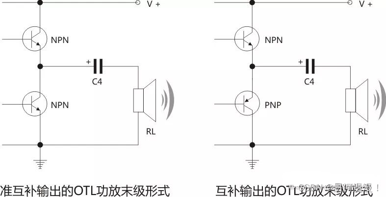
Unlike conventional push-pull amplifiers that use complementary pairs of NPN and PNP transistors, the JLH 1969 uses two identical NPN power transistors for the output [2]. This was a practical choice, as high-quality silicon NPN power transistors were more readily available and offered better performance and lower cost than their PNP counterparts in the 1960s [1].
Figure 3: Typical OTL output stages. The JLH 1969's use of two identical NPN transistors (left, quasi-complementary style) was a departure from the fully complementary (NPN/PNP) approach (right) that would later become standard [9].
To make this work, the driver stage (Tr2) must provide two signals of opposite phase. Linsley-Hood achieved this elegantly by taking one output from Tr2's collector and the other from its emitter [2]. The upper transistor (Tr3) functions as a collector load for the lower transistor (Tr4). This arrangement not only simplifies the parts list but also contributes to the amplifier's low distortion. As Linsley-Hood noted, the non-linearities of the two output transistors tend to cancel each other out, as one is turning full on while the other approaches cutoff [1].
Gain and Negative Feedback
A cornerstone of high-fidelity amplifier design is the use of negative feedback to reduce distortion, lower output impedance, and stabilize performance. The JLH 1969 employs a significant amount of feedback. The open-loop gain of the circuit is approximately 600 (or 55 dB) [1, 2]. The output signal is taken from the junction of the two output emitters and fed back to the emitter of the input transistor (Tr1) via resistor R5.
The closed-loop gain is determined by the ratio of the feedback resistors, specifically (R4 + R5) / R4. With the original component values, this results in a gain of about 13 (or 22 dB) [1, 2]. The difference between the open-loop and closed-loop gain gives a feedback factor of approximately 33-34 dB, a substantial amount that is responsible for the amplifier's impressively low distortion and an output impedance of about 160 milliohms [1].
The Bootstrap and Soft-Start Mechanisms
The circuit includes several other clever design elements. Capacitor C3, connected from the output to the junction of R1 and R2, forms a bootstrap circuit. This technique feeds a portion of the output signal back to the bias network of the driver stage. Its purpose is to make the driver transistor's collector load appear much larger than it actually is, allowing for a larger voltage swing and improving linearity and efficiency [2]. While effective, this is a feature some modern builders replace with a constant current source (CCS) for theoretically better performance [2, 10].
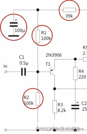
Figure 4: The unique biasing network for Tr1, featuring a 39k resistor and 100µF capacitor, creates a soft-start effect to protect the loudspeaker [2, 11].
Another subtle but important feature is the biasing network for the input transistor Tr1. The inclusion of a 39k resistor and a 100µF capacitor creates a slow-charging circuit at power-on. This causes the DC voltage at the output to rise gradually to its target of half the supply voltage over several seconds. This "soft-start" minimizes the turn-on "thump" that could otherwise damage the connected loudspeaker [2].
Linsley-Hood's design goal was to achieve a distortion level of less than 0.05% at full power, a very ambitious target for its time [3]. The published measurements show that the amplifier comfortably met this goal. The total harmonic distortion (THD) at 9 watts into a 15-ohm load was measured at just 0.06% with matched output transistors [1]. A key characteristic of this Class A circuit is that distortion decreases linearly as the output power is reduced. This is in contrast to Class B amplifiers, where crossover artifacts can cause distortion to rise at lower levels [1]. The residual distortion is predominantly benign second-order harmonic, which many listeners find to be musically pleasant and is often described as adding "warmth" and "richness" to the sound, reminiscent of tube amplifiers [1, 12].
The original design was specified for 10 watts of output power. The required supply voltage and quiescent current depend on the speaker's load impedance. For example, driving a 15Ω load to 10W requires a 36V supply and 0.9A of quiescent current. For an 8Ω load, it requires a 27V supply and 1.2A, and for a 3Ω load, a 17V supply and 2.0A [1]. This highlights the critical relationship between power supply, load, and thermal management in a Class A design. While 10 watts may seem low by modern standards, it is more than sufficient for high-efficiency speakers or for bi-amping systems where it might drive tweeters [3].
The Subjective "JLH Sound"
Beyond the specifications, the JLH 1969 is renowned for its subjective sound quality. It is often described as having a smooth, warm, and detailed character, frequently compared to that of a high-quality single-ended triode (SET) tube amplifier [12]. This is attributed to its simple signal path, lack of crossover distortion, and the nature of its harmonic distortion profile. The sound is often perceived as being very musical and non-fatiguing, making it a favorite for long listening sessions. Its ability to render vocals and acoustic instruments with a natural, lifelike texture is particularly praised by its proponents.
The enduring appeal of the JLH 1969 is fueled by the vibrant DIY audio community. Countless kits, PCBs, and fully assembled versions are available from vendors worldwide . For many, building a 1969 amplifier is a rite of passage, offering a rewarding project that results in a genuinely high-performance amplifier [15].
Over the decades, numerous modifications and improvements have been proposed. Common mods include:
Upgrading Components: Using modern, high-quality transistors, metal-film resistors, and audiophile-grade capacitors (especially for the input and output coupling capacitors) can yield significant sonic improvements.
Constant Current Source (CCS): Replacing the bootstrap circuit (C3 and associated resistors) with a dedicated CCS can improve linearity and power supply rejection [2].
DC-Coupled Output (OCL): Eliminating the large output coupling capacitor (C4) to create a direct-coupled (OCL) design. This requires adding a DC servo circuit to protect the speakers from DC offset but can improve bass response and transparency.
MOSFET Output Stage: Substituting the bipolar junction transistors (BJTs) in the output stage with MOSFETs. This creates a "1969M" variant, which can offer a different sonic signature and potentially operate in Class AB for higher efficiency [10].
Power Supply Enhancements: Using regulated power supplies or capacitor multipliers (electronic filters) can reduce noise and ripple, further cleaning up the sound [1].
Conclusion
The John Linsley-Hood 1969 Class A amplifier is more than just a vintage circuit; it is a testament to the power of elegant, thoughtful design. By prioritizing sonic purity and embracing simplicity, Linsley-Hood created an amplifier that not only challenged the performance of complex tube and solid-state designs of its day but also captured a musical quality that continues to resonate with listeners. Its legacy lives on not just in the yellowed pages of a 1969 magazine, but in the countless workshops and listening rooms around the world where enthusiasts continue to build, tweak, and enjoy its uniquely beautiful sound. It stands as a timeless reminder that in the pursuit of high fidelity, sometimes the simplest path is the most rewarding.







![[73]](https://www.kasuo.com/wp-content/uploads/2025/05/TDA7294-Pinout.jpg)
![[74]](https://www.kasuo.com/wp-content/uploads/2025/05/LM3886.jpg)