Single-Ended Output Transformers Core Size, DC Bias, and the Art of the Air Gap

Published by IWISTAO

A blog-form technical guide for builders of single-ended triode and pentode amplifiers

Figure 1. Why single-ended transformers must deal with continuous one-way DC flux while push-pull cores largely cancel it.

This blog is a faithful long-form adaptation of the source manuscript supplied by the user. It preserves the original technical argument, tables, and formulas while reshaping the material into a publishable article format.

Introduction

Among all parts of a vacuum-tube amplifier, the output transformer is both the most decisive and the most frequently misunderstood. That is especially true in single-ended (SE) amplifiers, where one output tube—or one paralleled output stage—continuously drives the primary winding with DC current present at all times. Unlike a push-pull stage, the transformer cannot assume that the net core magnetization will cancel. Instead, it must survive a standing DC bias current while still passing audio cleanly over the desired bandwidth.

The source article makes one central point: the defining feature of a true SE output transformer is the air gap. Without that gap, the DC component would push the magnetic core into saturation, leaving little room for the audio waveform. Everything else—core size, primary turns, inductance, low-frequency extension, winding geometry, weight, and cost—flows from that constraint.

In practical terms, the DC bias current may be modest, such as about 30 mA for a smaller directly heated triode, or well above 150 mA for large transmitting tubes such as the 845 or GM70. The stronger the standing DC magnetization, the larger the design penalty paid in core size and inductance management.

1. Why Single-Ended Transformers Are Fundamentally Different

In a push-pull output stage, two halves of the primary winding carry equal and opposite DC components. Because these magnetizing forces oppose one another, the transformer core sees very little net DC flux. That makes it possible to use an ungapped core and exploit nearly the full iron cross-section for AC signal swing.

A single-ended stage does the opposite. One active device establishes a quiescent DC current through the primary, and this current never reverses direction. The audio signal is therefore superimposed on top of a standing magnetic offset. The core is already biased before any music arrives.

The original manuscript compares the two topologies in concise engineering terms:

Parameter	Push-Pull	Single-Ended
DC flux in core	≈ 0 (cancels)	Significant
Air gap required	No	Yes—mandatory
Core utilization for audio	Near 100%	Reduced by DC reserve
Transformer size for a given power	Smaller	Typically 1.5× to 3× larger
Even-order distortion	Low	Second harmonic more prominent
Typical sonic reputation	Analytical / controlled	Often described as musical

The source article also illustrates the DC problem quantitatively with the standard field-intensity expression:

H_DC = (N_p × I_DC) / l_e

Here, N_p is the number of primary turns, I_DC is the quiescent current, and l_e is the effective magnetic path length. For a representative 300B SE example using roughly 2,800 primary turns, 80 mA of standing current, and an effective path length around 100 mm, the DC magnetizing field becomes large enough that an ungapped silicon-steel core would be driven into or beyond its usable region. The transformer would no longer behave as a linear audio device.

2. The Air Gap: The Essential Feature of an SE Output Transformer

The air gap solves the DC saturation problem by inserting a controlled non-magnetic reluctance into the magnetic circuit. Air has a relative permeability of about 1, enormously lower than that of transformer steel. As a result, even a small physical gap dominates the reluctance of the magnetic path.

Figure 2. Introducing a gap sharply reduces effective permeability, but it also prevents the standing DC bias from driving the core into saturation.

The source text uses the familiar approximation that the effective permeability of a gapped core is roughly proportional to l_e / l_g when the intrinsic permeability of the steel is much higher than that ratio. This is the heart of the tradeoff: the gap saves the core, but it also lowers primary inductance. Since low-frequency response depends on inductance, every increment of gap has a price.

The article further gives the design equation for the required total gap length:

l_g = (μ₀ × N_p × I_DC) / B_max − l_e / μ_r

Using the worked 300B example from the manuscript—EI-66 core, about 2,800 primary turns, 80 mA DC, and a chosen DC flux density target around 0.9 T—the total gap comes out close to 0.30 mm. For a conventional EI stack, that corresponds to about 0.15 mm shim thickness on each side.

3. Core Size and Output Power

The next major theme of the original article is that single-ended transformers are not sized by power alone. They must simultaneously survive DC bias and still provide enough primary inductance for the target low-frequency cutoff. A useful rule from the manuscript is that core area and window area together set the practical power-handling envelope, and the usable output tends to scale approximately with the square of the core cross-section area.

Figure 3. Typical SE power capability rises steeply as core cross-section area increases.

Core	A_e (cm²)	Typical P_out (W)	Common tubes	I_DC (mA)	Gap total (mm)
EI-48	1.44	0.5–1.5	45, 71A, PX4	25–40	0.05–0.10
EI-57	2.04	1.5–3	2A3, 45, EC8010	35–60	0.10–0.15
EI-66	2.72	3–6	2A3, 300B, PX25	60–90	0.15–0.25
EI-76	3.61	5–9	300B, 6L6 SE, EL34 SE	70–100	0.20–0.30
EI-86	4.62	8–14	845, 211, 300B parallel	90–130	0.25–0.40
EI-96	5.76	12–20	845, GM70, 211	100–150	0.30–0.50
EI-114	8.12	18–30	Parallel 845, GM70×2	150–250	0.40–0.70

One practical design lesson emerges clearly: in SE work, 'more iron' is rarely wasted. Larger cores allow more DC headroom, more low-frequency inductance, and lower flux density stress for a given power level. That is why high-quality 845, 211, and GM70 transformers quickly become physically large and expensive.

The source manuscript also discusses toroidal and cut-core approaches. Because a toroid does not naturally have a joint where a gap can be inserted, manufacturers must cut the core and insert a precision spacer or gap it at manufacture. Amorphous and nanocrystalline materials can improve inductance for a given size, but they do not remove the need to manage DC bias carefully.

4. Primary Inductance: The Real Gatekeeper of Bass Performance

The blog source makes a point that many hobbyists overlook: surviving DC is not enough. An SE transformer also needs adequate primary inductance, because the primary inductance and the source impedance of the output tube form the low-frequency high-pass behavior of the output stage.

The lower cutoff frequency can be approximated by:

f_L = (R_a || R_L′) / (2π × L_p)

For a 300B example with plate resistance around 700 Ω and a reflected primary load of 5 kΩ, the effective source resistance becomes about 609 Ω. Hitting 20 Hz therefore requires a minimum primary inductance a little under 5 H, while more conservative designs aim for roughly 5–8 H or more to preserve authority in the lowest octave.

Once the gap is chosen, the achievable inductance is approximately:

L_p = (μ₀ × N_p ² × A_e) / (l_g + l_e / μ_r)

The original calculation for an EI-66 300B transformer gives an inductance of roughly 10 H with a 0.30 mm total gap—comfortably above the minimum and consistent with strong low-frequency extension.

Tube	R_a (Ω)	Typical Z_a (Ω)	Min L_p @20Hz (H)	Recommended L_p (H)	Typical N_p
45	1,600	1,600	12.7	20–30	3,500–4,500
2A3	800	2,500	6.4	10–18	2,500–3,500
300B	700	3,500–5,000	5.6	8–15	2,200–3,200
845	1,700	5,000–7,000	13.5	20–35	3,000–4,000
211	1,650	5,000–7,000	13.1	20–35	3,000–4,000
GM70	2,000	3,500–5,000	15.9	25–40	3,500–4,500
EL34 (triode SE)	1,000	3,000	7.9	12–20	2,500–3,200
KT88 (pentode SE)	13,000	3,500	17.2	30–50	3,500–5,000

5. Turns Ratio, Secondary Design, and Load Matching

The original manuscript next walks through the familiar impedance-transformation relationship between primary and secondary:

n = √(Z_a / Z_L)

For a 300B driving an 8 Ω loudspeaker from a 3.5 kΩ primary load, the required turns ratio is about 20.9:1. With roughly 2,800 primary turns, that yields about 134 turns on the 8 Ω secondary. From there, wire size is chosen according to current density. In the example, an 8 W / 8 Ω load produces about 1 A RMS, implying a secondary conductor area near 0.286 mm².

The source also notes that many commercial transformers include 4 Ω, 8 Ω, and 16 Ω taps. These are established by the square-law relationships of turns and impedance, not by arbitrary choice. Correct load matching is central to getting the intended power, distortion, and damping behavior from the output tube.

6. High-Frequency Response: Leakage Inductance and Distributed Capacitance

At the top end, transformer behavior is dominated not by primary inductance but by leakage inductance and distributed capacitance. The source article explains the tradeoff elegantly: better interleaving improves coupling and pushes high-frequency rolloff upward, but additional layering can increase interwinding capacitance.

Figure 4. Interleaving the primary and secondary reduces leakage inductance and extends high-frequency bandwidth, though usually at the cost of increased distributed capacitance.

Winding configuration	Relative L_leak	Typical HF -3 dB	Relative C_dist
Simple P-S	1×	30–60 kHz	1×
½P – S – ½P	~0.25×	80–150 kHz	2×
¼P – S – ½P – S – ¼P	~0.06×	150–300 kHz	4×

In other words, transformer design is always a controlled compromise. Bass extension, DC tolerance, copper loss, leakage inductance, capacitance, and manufacturability all pull in different directions. Good transformers are not optimized by a single variable; they are balanced.

7. Worked Design Examples from the Source Article

To make the theory concrete, the original manuscript provides three useful design snapshots. They are reproduced below in blog form.

Design	Core	Primary Z	I_DC (mA)	Primary turns	Gap total (mm)	L_p (H)	Low -3 dB	Weight
300B SE	EI-66 M6	3,500 Ω	80	2,700	0.30	~10	~9 Hz	~450 g
845 SE	EI-96 GO steel	6,000 Ω	75	3,400	0.25	~22	~10 Hz	~950 g
2A3 SE	EI-57 M6	2,500 Ω	60	2,200	0.15	~7	~14 Hz	~280 g

These examples reinforce the article's central theme. A 300B transformer that looks modest on paper still needs careful gap management and enough turns to achieve around 10 H. Step up to an 845, and both core mass and winding effort rise dramatically. Drop down to a 2A3, and everything becomes a bit more compact, but the same magnetic logic still applies.

8. Practical Mistakes Warns Against

• Under-gapping the core. This leaves the iron too close to saturation and causes abrupt distortion on peaks.
• Over-gapping the core. This preserves DC headroom but reduces primary inductance, weakening bass and forcing more turns.
• Ignoring primary DC resistance. Excess winding resistance wastes voltage, raises copper loss, and degrades performance.
• Using push-pull transformers in SE circuits. A non-gapped PP transformer is not a substitute for a proper SE unit.
• Ignoring tube plate resistance. Low-frequency requirements depend on the source impedance of the tube, not just on the nominal primary load.

We also stresses lamination orientation, especially with grain-oriented steel, and reminds builders that winding resistance rises with temperature. Those effects do not invalidate the basic design equations, but they matter in serious builds and should not be treated as afterthoughts.

10. Advanced Notes

The manuscript closes its technical discussion with several advanced topics that deserve mention in a complete blog version.

• Feedback windings can be added to improve damping and extend bandwidth, but phase management becomes critical at high frequency.
• Single-ended pentodes can use ultralinear-style screen taps, often around 25–35% of the primary winding, to trade gain for lower distortion.
• Copper resistance rises about 0.393% per °C, so hot transformers behave differently from cold bench measurements.
• At audio frequencies, hysteresis is a major component of core loss; careful material choice and conservative flux density still matter.

Conclusion

The strength of the article lies in how consistently it ties every design choice back to one immutable fact: a single-ended output transformer must carry DC. Once that is accepted, the rest of the design becomes a balancing act among saturation margin, available AC swing, primary inductance, copper loss, leakage inductance, capacitance, and cost.

In concise rule-of-thumb form, the manuscript leaves the reader with three memorable ideas. First, every watt of serious low-frequency SE output requires substantial iron. Second, the air gap is not an optional tweak but the defining feature of the topology. Third, primary inductance must be chosen with the tube's source resistance in mind, not by catalog optimism alone.

For builders, that means the output transformer is never the place to economize blindly. In single-ended design, the iron is not merely a passive coupler. It is one of the principal determinants of the amplifier's final sound, power delivery, and bandwidth.

Shop Output Transformers

Find More

• The Ultimate Upgrade: Exploring Amorphous C-Core Output Transformers for the 300B Tube Amp
• The Heart of Harmony: A Deep Dive into Push-Pull Output Transformers
• A DIY Guide: Building a Power Transformer for an EL34B Push-Pull Tube Amplifier

References

The following references are reproduced from the source manuscript and retained here to preserve attribution and technical lineage.

1. Turner, Bruce. "Single-Ended Output Transformer Calculator and Design Guide." Turner Audio. https://turneraudio.com.au/se-output-trans-calc-1.html
2. Merlin, Gary. "The Valve Wizard: Single-Ended Output Stages." https://www.valvewizard.co.uk/se.html
3. Sowter Transformers. "Single-Ended Output Transformers Product Range." https://www.sowter.co.uk/single-ended-output-transformers.php
4. Lundahl Transformers. "Tube Amplifier Output Transformers." https://www.lundahltransformers.com/tube-output/
5. Hashimoto Electric. "SE Output Transformer Specifications — H Series." https://acoustic-dimension.com/hashimoto/hashimoto-output-transformers-single-ended.htm
6. Hammond Manufacturing. "Audio Output Transformers — SE Series." https://www.hammfg.com/electronics/transformers/audio
7. Ridley, Ray. "Air Gap Design for Inductors with DC Bias." Ridley Engineering. https://www.ridleyengineering.com/design-center-ridley-engineering/39-magnetics/128-air-gap-design-for-inductors-with-dc-bias.html
8. van der Veen, Menno. "Modern High-End Valve Amplifiers Based on Toroidal Output Transformers." Elektor, 1999.
9. RCA Corporation. "Radiotron 300B Data Sheet." 1938. http://www.duncanamps.com/tube/300b.html
10. Jones, Morgan. "Valve Amplifiers, 4th Edition." Newnes/Elsevier, 2012.
11. Blencowe, Merlin. "Designing Tube Preamps for Guitar and Bass." Wem Publishing, 2009.
12. Langford-Smith, F. (ed.). "Radiotron Designer's Handbook, 4th Edition." Wireless Press, 1952. https://www.tubebooks.org/technical_files/RDH4.pdf
13. Crowhurst, Norman H. "Audio Transformer Design Manual." Gernsback Library, 1958.
14. Wolpert, David. "Design and Construction of High-Performance Audio Transformers." Glass Audio, Vol. 12(3), 2000.
15. National Magnetics Group. "Amorphous and Nanocrystalline Core Materials for Audio Transformers." https://www.natmag.com/

Principles and Design Analysis of Electroacoustic Conversion in Moving-Coil Loudspeakers

Published by IWISTAO

Speakers are indispensable components in audio systems, and their performance directly determines sound reproduction quality and listening experience. Among common speaker types, moving-coil loudspeakers are the most common. This paper explores in depth the electroacoustic conversion principle and provides detailed formula derivations and design analysis.

I. Basic Structure and Working Principle of Moving-Coil Loudspeakers

A typical moving-coil loudspeaker consists of the following key components:

• Voice coil: after energization, it generates a magnetic field and interacts with the magnetic circuit;
• Magnetic circuit system: provides a constant magnetic field;
• Diaphragm: driven by the voice coil to vibrate, pushing air to produce sound;
• Suspension system: including spider and surround, ensuring vertical motion of the voice coil while limiting lateral displacement.

The working principle of a moving-coil loudspeaker is as follows: when alternating current (audio signal) is input to the voice coil, electromagnetic induction causes the voice coil and magnetic circuit to generate an interaction force that drives the diaphragm to move back and forth; diaphragm vibration pushes air to radiate sound waves, realizing conversion from electrical energy to acoustic energy.

II. Electromagnetic Transduction Process and Formula Derivation

The electroacoustic conversion of moving-coil loudspeakers is essentially an electromagnetic energy conversion process. According to the Lorentz force law (Lorentz Force Law), the force acting on the voice coil can be expressed as:

F = B · l · i

where:

• F: electromagnetic force acting on the voice coil (unit: N)
• B: magnetic flux density in the gap magnetic field (unit: T)
• l: effective conductor length of the voice-coil winding (unit: m)
• i: current through the voice coil (unit: A)

The electromagnetic force on the voice coil drives diaphragm vibration, and the diaphragm motion equation can be described by the classical mass-spring-damper system:

m d²xdt² + R_m dxdt + Kx = F

where:

• m: equivalent mass of the loudspeaker vibration system (unit: kg)
• R_m: mechanical damping coefficient (unit: N·s/m)
• K: stiffness coefficient of the suspension system (unit: N/m)
• x: displacement of the voice-coil/diaphragm system (unit: m)

Substituting the electromagnetic force expression into the above equation yields:

m d²xdt² + R_m dxdt + Kx = Bli

This is the fundamental differential equation of loudspeaker electromechanical coupling.

III. Electrical Equivalent Impedance Model of the Loudspeaker

The loudspeaker voice coil also has electrical characteristics, which can be represented by an electrical equivalent impedance model:

The voltage-current relationship of the voice coil can be expressed as:

u(t) = R_ei(t) + L_e di(t)dt + e(t)

where:

• u(t): loudspeaker input voltage (unit: V)
• R_e: voice-coil resistance (unit: ohm)
• L_e: voice-coil inductance (unit: H)
• e(t): back electromotive force (Back EMF)

Because the vibrating voice coil cuts magnetic field lines and generates back EMF, according to Faraday's law of electromagnetic induction:

e(t) = Bl dxdt

In frequency-domain analysis, complex numbers are used:

X(ω), I(ω), U(ω)

satisfy:

U(ω) = (R_e + jωL_e)I(ω) + jωBlX(ω)

and the mechanical equation in the frequency domain is:

(jω)²mX(ω) + jωR_mX(ω) + KX(ω) = BlI(ω)

Combining the above two equations and eliminating displacement, the loudspeaker electrical input impedance expression can be obtained:

Z(ω) = R_e + jωL_e + (Bl)²R_m + j(ωm - Kω)

IV. Loudspeaker Sensitivity and Efficiency Analysis

An important loudspeaker metric, sensitivity, is defined as the sound pressure level at a specific distance under a specified input voltage, usually expressed in dB SPL:

Loudspeaker efficiency is defined as output acoustic power to input electrical power ratio:

η = P_acousticP_electric × 100%

Loudspeaker output acoustic power can be determined through the concept of diaphragm radiation acoustic impedance:

P_acoustic = 12R_rad(ω)v²

where:

• R_rad(ω): real part of the loudspeaker radiation acoustic impedance, representing resistance to acoustic radiation (unit: N·s/m)
• v: diaphragm velocity amplitude (unit: m/s)

Based on the relationship between diaphragm velocity and displacement, and the above relationship among displacement, current, and input voltage, one can further calculate loudspeaker sensitivity and efficiency in detail.

V. Design Optimization Considerations

In practical design, the following factors need to be considered comprehensively to optimize performance:

• Magnetic circuit design: increasing magnetic flux density B can increase electromagnetic conversion efficiency;
• Voice-coil design: reasonably select conductor length and wire diameter to optimize impedance matching;
• Diaphragm design: reducing mass m improves sensitivity while balancing stiffness and damping characteristics;
• Suspension system design: appropriate elastic coefficient K and damping R_m, to achieve reasonable frequency-response characteristics and stability.

VI. Summary

The electroacoustic conversion process of moving-coil loudspeakers is essentially a mechanically vibrating system driven by electromagnetic force; through systematic formula derivation and analysis, one can clearly understand the loudspeaker working principle and the influence of key design parameters. Loudspeaker design and optimization are a multivariable trade-off process requiring comprehensive consideration of electrical, magnetic-circuit, mechanical, and acoustic factors to achieve ideal sound reproduction state.

Shop Speaker Units

Find More

The Heart of Your Sound System: A Deep Dive into Speaker Cones

Understanding Different Types of Loudspeaker Drivers

LS3/5A Cabinet Acoustic Damping Application Engineering and Listening Notes

The Science of Speaker Isolation Spikes

Published by IWISTAO

How tiny metal cones beneath your speakers can transform muddy vibrations into crystalline sound — and why physics demands them.

Every speaker vibrates. That's the point — it converts electrical signals into mechanical movement to produce sound waves. But not all vibration is created equal, and the energy your speakers dump into shelves, stands, and floors is energy that isn't becoming music.

Speaker isolation spikes — also called decoupling feet, isolation cones, or audiophile spikes — are small pointed metal accessories that attach to the bottom of your speakers. They look deceptively simple, almost decorative. But their design is rooted in basic physics, and their effect on sound quality can be surprisingly dramatic.

In this article, we'll explore how isolation spikes work, why they matter, and how to choose the right set for your setup.

Fig. 1 — Comparison: vibration transfer with and without isolation spikes

Why Speakers Vibrate Their Environment

A speaker driver works by moving a cone back and forth rapidly to push air. Newton's Third Law applies: for every action, there's an equal and opposite reaction. As the cone pushes air forward, the speaker cabinet is pushed backward. This reactive force travels through the cabinet, into whatever it's sitting on, and into the structure of your room.

The result? Your bookshelf becomes a secondary speaker. Your desk resonates at certain frequencies. Your floor joists hum along with the bass. All of this adds coloration — unwanted resonances that smear the sound, muddy the bass, and reduce clarity in the midrange.

This is especially problematic with:

• Nearfield monitors on desks (desk resonance is a notorious problem)
• Floorstanding speakers on wooden floors (floor coupling adds bass bloat)
• Bookshelf speakers on shelves (the shelf acts as a soundboard)
• Subwoofers anywhere (massive low-frequency energy seeks every path)

The Physics of Isolation: Point Contact

Isolation spikes work on a beautifully simple principle: minimizing the contact area between two surfaces.

A flat-bottomed speaker sitting on a flat shelf has a large contact patch — perhaps dozens of square centimeters. Every square centimeter is a pathway for vibration to travel. The spike reduces this to a point contact, typically less than 1 mm² per spike.

This has two effects:

1. Reduced transmission area — Less physical contact means fewer pathways for mechanical energy to escape the cabinet.
2. Increased pressure at the contact point — The entire weight of the speaker concentrates on a tiny point, which can slightly "dig into" the surface, creating a stable, anchored position that resists lateral movement.

The Analogy: Imagine pushing a balloon against a wall with your whole palm versus with a single fingertip. With the palm, the energy transfers broadly. With the fingertip, the balloon deforms locally but the wall behind it feels far less force. The spike is the fingertip.

Fig. 2 — Contact area comparison: flat bottom vs. spike point contact

Coupling vs. Decoupling: A Critical Distinction

Not all spike setups work the same way. There are actually two opposing philosophies, and choosing the right one depends on your situation:

Coupling (Spikes Into a Hard Surface)

When spikes press directly into a hard surface like stone, concrete, or a metal plate, they couple the speaker to the surface — locking it rigidly in place. The theory here is that a massive, rigid surface (like a concrete floor) will absorb and dissipate vibration more effectively than the speaker cabinet alone. The speaker becomes an extension of the mass.

This is the traditional approach for floorstanding speakers on concrete or tiled floors.

Decoupling (Spikes on Isolation Pads)

When spikes sit on rubber, sorbothane, or felt pads, they decouple the speaker from the surface. The spike concentrates the weight, and the compliant material beneath absorbs vibration before it reaches the surface. This is the preferred approach for desk setups, wooden floors, and shelf-mounted speakers.

Rule of Thumb: Hard, massive floor → couple with spikes directly. Flexible surface (desk, wood floor, shelf) → decouple with spikes + pads. Getting this wrong can actually make things worse.

Spikes → Hard Floor (Coupling)

Spikes → Pad → Surface (Decoupling)

Audible Benefits: What You'll Actually Hear

The improvements from proper isolation are not subtle once you know what to listen for. Commonly reported changes include:

1. Tighter, More Defined Bass

When your desk or floor vibrates in sympathy with bass notes, it adds a boomy, one-note quality to the low end. Isolation removes this secondary resonance, revealing the actual texture and pitch definition in bass instruments. Kick drums get punch instead of thud. Bass guitar lines become individually discernible.

2. Improved Stereo Imaging

Vibration-induced cabinet movement smears the stereo image. When speakers are firmly anchored (coupled) or properly isolated (decoupled), the soundstage snaps into focus. You'll hear instruments placed more precisely between and beyond the speakers. Depth perception improves.

3. Cleaner Midrange

Desk and shelf resonances often fall squarely in the midrange (200 Hz–800 Hz), adding a nasal, boxy coloration. Isolation can dramatically clean this up, making vocals more natural and guitars more detailed.

4. Reduced Listener Fatigue

All that unwanted resonance adds up to a form of distortion your brain has to work to filter out. Removing it makes extended listening sessions less tiring — a benefit that's hard to measure but easy to feel.

Types of Isolation Spikes and Feet

Type	Material	Best For
Steel Cone Spikes	Hardened steel or brass	Floorstanding speakers on hard floors
Aluminum Isolation Feet	Anodized aluminum	Bookshelf speakers, nearfield monitors
Sorbothane Hemispheres	Sorbothane (viscoelastic polymer)	Desk setups, decoupling on any surface
Spring Isolation Platforms	Steel springs + mass plate	Turntables, sensitive electronics, speakers
Spike + Disc Combos	Steel spikes + matching cups/discs	Protecting surfaces while coupling

DIY Solutions That Actually Work

You don't necessarily need to spend a fortune. Some effective DIY approaches include:

• Cork pads: Dense cork coasters or tiles cut to size provide decent decoupling for nearfield monitors. Cost: nearly free.
• Rubber washing machine pads: Anti-vibration pads designed for washing machines are cheap, dense, and surprisingly effective under speakers.
• Tennis balls (halved): A classic studio trick — cut tennis balls in half and place them under speakers. The air-filled rubber provides excellent isolation. Not pretty, but effective.
• Concrete pavers + foam: Place a heavy concrete paver on foam pads, then put your speakers on the paver. This adds mass (inertia) while isolating from the desk. A favorite among home studio engineers.

Studio Pro Tip: The "concrete paver on foam" trick is used in professional studios worldwide. A 2" thick concrete slab on four small foam pads can outperform many commercial isolation products at a fraction of the cost. The mass resists movement; the foam absorbs vibration. Simple physics, outstanding results.

Installation Tips

1. Three points are better than four — A three-point stance is inherently stable on uneven surfaces. If your speakers have four spike mounts, consider using three spikes (two front, one rear) for guaranteed stability.
2. Use spike discs on wood floors — Bare spikes will dent and scratch hardwood. Metal or ceramic discs distribute the load and protect the surface.
3. Level your speakers first — Spikes amplify any tilt. Make sure your stands or surfaces are level before installing.
4. Tighten gradually — Threaded spikes should be tightened evenly, a few turns at a time, alternating between corners.
5. Test before and after — Play a track you know well. Listen for changes in bass definition, midrange clarity, and stereo width. The difference should be audible.

Fig. 3 — Installation guide: from threaded holes to final placement

Common Myths and Misconceptions

"Spikes always improve sound"

Not universally. Spikes on a suspended wooden floor can actually increase floor resonance by coupling the speaker directly to a resonant surface. In this case, decoupling (spikes on pads, or flat isolation feet) is the better choice. Context matters.

"More expensive spikes sound better"

Diminishing returns kick in fast. A $20 set of steel spikes provides 90% of the benefit of a $200 set of machined brass cones. The physics of point contact doesn't change much with material — what changes is build quality, aesthetics, and thread compatibility.

"Spikes are just audiophile snake oil"

While some audiophile products push the boundaries of credulity, isolation spikes are grounded in straightforward physics. The principle of reducing contact area to minimize vibration transfer is well-established in mechanical engineering. The effect is measurable — accelerometer tests on speaker cabinets consistently show reduced surface vibration when spikes are properly deployed.

The Bottom Line

Speaker isolation spikes are one of the most cost-effective upgrades you can make to an audio system. They address a real, physics-based problem with a simple, elegant solution. Whether you're running a pair of studio monitors on a desk or floorstanding speakers in a living room, properly implemented isolation will tighten your bass, clarify your mids, and reveal details in your music that were previously masked by resonant surfaces.

The key is understanding your specific situation: couple on hard floors, decouple on flexible surfaces, and always test with your own ears. The best spike is the one that solves your particular vibration problem — and sometimes that's a $2 tennis ball.

Shop Speaker Shock Spike and Mat Kit

Find more

Decoding the Current: A Comprehensive Guide to Speaker Cables

References

1. Toole, Floyd E. Sound Reproduction: The Acoustics and Psychoacoustics of Loudspeakers and Rooms. Focal Press, 3rd edition, 2017. — Comprehensive treatment of loudspeaker-room interaction and vibration coupling.
2. Harman International. "Loudspeaker and Headphone Handbook." harman.com — Technical resources on speaker design and measurement.
3. Sorbothane, Inc. "Sorbothane Technical Guide." sorbothane.com — Material properties and damping characteristics of viscoelastic polymers used in isolation products.
4. Ethan Winer. "Acoustic Treatment and Design for Recording Studios and Listening Rooms." ethanwiner.com/acoustics.html — Practical guide to room acoustics including speaker isolation.
5. Genelec. "Monitoring Guide: Speaker Placement and Isolation." genelec.com — Professional studio monitor manufacturer's recommendations on decoupling.
6. Sound On Sound Magazine. "Speaker Isolation: Does It Work?" — Independent testing and measurements of various isolation products. soundonsound.com
7. Newton, Isaac. Philosophiæ Naturalis Principia Mathematica, 1687. — Third Law of Motion as applied to speaker reactive forces.

Software Defined Radio (SDR): A Complete Practical Guide to I/Q Sampling, Portable SDR Receivers, Antennas, and Real-World Shortwave Listening

Published by IWISTAO

A comprehensive guide covering what SDR is, how it works, why I/Q sampling matters, how the Malahit DSP SDR V3 fits into modern radio listening, and how to choose the right antenna for better shortwave reception.


Figure 1. A modern SDR receiver displays a live spectrum and waterfall, making radio signals visible as well as audible.

Contents

1. What Is a Software Defined Radio?
2. Why SDR Is Different from Traditional Radios
3. The Core Technology: I/Q (Quadrature Sampling)
4. Typical SDR Signal Processing Chain
5. The Malahit DSP SDR V3 Portable Receiver
6. Inside the Malahit SDR Architecture
7. What Signals Can SDR Receivers Receive?
8. Active Antenna Amplifiers
9. Best Antennas for Shortwave Reception
10. Why MLA-30 Performance Varies
11. Practical SDR Listening Advice
12. FAQ
13. Related Products
14. Further Reading
15. References

Software Defined Radio, usually called SDR, has fundamentally changed the way radio enthusiasts, experimenters, and shortwave listeners receive signals. What once required a chain of specialized analog circuits can now be performed largely through digital signal processing and software algorithms.

With a traditional radio receiver, users normally tune to one frequency and listen. With an SDR, however, the radio spectrum becomes visual, interactive, and much more flexible. You can see carriers, detect interference, change filters in real time, switch demodulation modes instantly, and analyze weak signals in ways that were once limited to expensive communications receivers and laboratory equipment.

This guide explains the principles behind SDR, the importance of I/Q sampling, the role of portable receivers such as the Malahit DSP SDR V3, and the practical reality that antennas often matter more than the receiver itself—especially for shortwave listening.

1. What Is a Software Defined Radio?

Software Defined Radio is a radio communication system in which many signal-processing functions traditionally performed by dedicated hardware are instead performed by software.

In a traditional analog radio, the signal path typically follows this chain:

Antenna → RF Amplifier → Mixer → Intermediate Frequency Filter → Demodulator → Audio Amplifier

Each block performs a dedicated hardware role. If you want to change how the radio behaves, you often need to change the hardware design itself.

In an SDR receiver, the architecture shifts much of that complexity into software:

Antenna → RF Front End → Analog-to-Digital Converter → Digital Signal Processing → Audio Output

Because of this approach, a single SDR platform can support multiple radio modes and signal-processing features through firmware or software, without requiring a different analog receiver design for each task.

Figure 2. SDR shifts many traditional radio functions from fixed hardware into flexible digital signal processing.

2. Why SDR Is Different from Traditional Radios

One of the most transformative advantages of SDR is that it makes the radio spectrum visible. Instead of tuning blindly, the user sees stations appear as spectral peaks and watches signal history unfold in the waterfall.

Figure 3. The spectrum and waterfall view help users identify signals, interference, fading, and band activity in real time.

This visualization provides several practical benefits:

• Signals can be identified much faster.
• Interference sources become easier to recognize.
• Fading, drift, and overload are more obvious.
• Multiple stations can be observed across a band segment at once.
• Weak carriers become visible even before they are fully audible.

For shortwave listeners, this is especially useful because propagation changes throughout the day. SDR makes it possible to respond to those changes in a far more informed and efficient way than with a traditional analog receiver.

3. The Core Technology: I/Q (Quadrature Sampling)

One of the most important concepts in SDR is quadrature sampling, usually referred to as I/Q sampling.

In SDR, the receiver measures two related signal components that differ by 90 degrees in phase:

• I (In-phase)
• Q (Quadrature)

Mathematically, these can be represented as:

Formula Image 1

Formula Image 2

Together they form a complex signal representation:

Formula Image 3

Figure 4. I/Q sampling preserves amplitude and phase information, enabling advanced digital demodulation and spectrum analysis.

By preserving both components, the receiver retains enough information to reconstruct the signal in software. This is what makes digital filtering, FFT spectrum displays, frequency shifting, AM detection, SSB demodulation, and many other SDR features possible.

In practical terms, I/Q is one of the reasons SDR behaves less like a conventional radio and more like a flexible signal-processing instrument.

4. Typical SDR Signal Processing Chain

Although implementations vary, most SDR receivers follow a similar signal flow:

Figure 5. The SDR signal chain begins at the antenna and ends in digital demodulation and audio or data output.

1. Antenna: receives electromagnetic energy from the environment.
2. RF Front End: provides filtering, protection, and sometimes amplification.
3. ADC or Tuner Stage: converts or prepares the signal for digital sampling.
4. Digital Signal Processing: performs filtering, gain control, demodulation, FFT analysis, and audio recovery.
5. Output Stage: sends audio to headphones or a speaker, or exports data to software tools.

This architecture allows one receiver to support many listening tasks, from AM and FM to SSB, CW, and digital modes, using software-defined methods rather than fixed analog circuitry.

5. The Malahit DSP SDR V3 Portable Receiver

The Malahit DSP SDR V3 has become one of the most talked-about portable SDR receivers because it offers a self-contained SDR experience without requiring a PC. For many users, that is its biggest attraction.

Figure 6. The Malahit DSP SDR V3 integrates spectrum display, DSP processing, and battery-powered operation in a handheld format.

Typical strengths include:

• Portable all-in-one SDR receiver design
• Real-time spectrum and waterfall display
• Support for AM, FM, SSB, and CW demodulation
• Battery-powered field operation
• Compact size suitable for travel and portable listening

In effect, it brings many of the visual and analytical advantages of desktop SDR into a handheld format, making it highly attractive to shortwave listeners, radio experimenters, and portable monitoring enthusiasts.

6. Inside the Malahit SDR Architecture

Internally, a portable SDR such as the Malahit typically includes several major functional blocks:

• RF input stage
• Front-end filtering and signal conditioning
• Tuner or sampling section
• Main DSP or high-speed microcontroller
• Audio codec and output stage
• Battery and power-management circuitry
• Display and user-interface subsystem

Figure 7. An example of internal architecture of a portable SDR receiver: RF front end, digital processing, audio stage, and power management.

The internal signal path can be summarized like this:

Antenna
↓
RF filtering
↓
Tuner or ADC
↓
I/Q digital processing
↓
Demodulation
↓
Audio output

In SDR systems, firmware matters because it directly influences behavior such as AGC response, filter performance, UI responsiveness, waterfall rendering, and sometimes even subjective listening quality.

7. What Signals Can SDR Receivers Receive?

Depending on hardware capability and the antenna system, SDR receivers can cover a remarkably wide range of listening activities.

AM broadcast

FM broadcast

Shortwave broadcast

Amateur radio

Aviation communications

Marine communications

CW and SSB utility signals

Digital modes

ADS-B aircraft data

Weather and satellite-related signals

This flexibility is one of the strongest reasons SDR has become so popular. A single device can serve as a general coverage receiver, learning tool, and visual signal analyzer all at once.

8. Active antenna amplifier

An active antenna amplifier, often called an LNA (Low Noise Amplifier), is used near the antenna to boost weak signals before they are weakened by feedline loss.

Figure 8. A wideband LNA can help weak-signal reception, but too much gain may cause overload and intermodulation.

Antenna
↓
Low Noise Amplifier
↓
Coaxial Cable
↓
SDR Receiver

Potential benefits include:

• Compensation for coaxial cable loss
• Improved weak-signal reception
• Better performance from physically small antennas

Potential drawbacks include:

• Receiver overload
• Raised noise floor
• Intermodulation products
• False or spurious signals

In practice, an amplifier is not a magic upgrade. A better antenna in a quieter location often improves reception more than simply adding gain.

9. Best Antennas for Shortwave Reception

For shortwave and HF listening, the antenna system often matters more than the receiver itself. Three practical antenna categories are especially relevant to SDR users.

9.1 Long Wire Antenna

Figure 9. A long wire antenna remains one of the most economical and effective ways to improve shortwave reception.

A simple long wire setup often looks like this:

10–20 m wire
↓
9:1 balun or matching transformer
↓
Receiver

Advantages:

• Strong signal capture
• Very low cost
• Good DX capability
• Simple to build and install

9.2 Magnetic Loop Antenna

Figure 10. Magnetic loop antennas are often favored in noisy locations because they can improve signal-to-noise ratio.

Advantages:

• Compact physical size
• Better performance in noisy urban settings
• Directional nulling of interference
• Well suited to balconies and limited spaces

9.3 Active Mini-Whip Antenna

Figure 11. Active mini-whip antennas are compact, but their effectiveness depends heavily on grounding and installation environment.

Advantages:

• Very small size
• Wide frequency coverage
• Convenient where installation space is extremely limited

Disadvantages:

• More vulnerable to local electrical noise
• Grounding is critical
• Can be less forgiving than a loop or outdoor wire for HF reception

10. Why MLA-30 Performance Varies

Many beginners say the MLA-30 is noisy, while experienced listeners sometimes use it quite successfully. The difference usually comes down to installation quality rather than the loop itself.

Figure 12. An MLA-30 installed outdoors and away from household electronics can perform far better than the same loop used indoors.

Indoor Installation

This is one of the most common reasons for poor results. Indoor environments are full of RF noise from LED lamps, routers, chargers, televisions, computers, and switching power supplies.

Proximity to Electronics

Even if the loop is near a window, it may still be too close to the building’s wiring and noise sources. Moving the antenna outdoors often reduces the noise floor dramatically.

Incorrect Orientation

Magnetic loops have directionality. Rotating the loop can null a noise source or improve signal readability.

Poor Power Quality

Since the MLA-30 uses an active amplifier and bias-tee arrangement, a noisy USB power source can inject additional interference into the receiving system.

Too Much Gain

Increasing receiver gain does not necessarily improve reception. It may only brighten the waterfall and raise the apparent noise floor.

Practical takeaway: When an MLA-30 sounds noisy, the real problem is often the surrounding electrical environment, not the antenna design itself.

11. Practical SDR Listening Advice

If you want better real-world SDR reception, especially on shortwave, the following priorities are usually more effective than simply buying more gain or a more expensive radio:

1. Improve antenna placement. Outdoor placement usually helps more than adding gain.
2. Reduce local noise sources. Distance from household electronics matters enormously.
3. Use moderate gain settings. Avoid overloading the receiver.
4. Experiment with antenna direction. Especially important for magnetic loops.
5. Learn the waterfall display. It reveals fading, overload, interference, and signal behavior.

In many cases, a modest SDR connected to a well-installed antenna will outperform a more expensive receiver used in a poor RF environment.

FAQ

What is the biggest advantage of SDR compared with a traditional radio?

SDR combines flexible digital signal processing with live spectrum and waterfall visualization, allowing one receiver to support multiple modes and provide much greater signal insight.

Why is I/Q sampling important in SDR?

I/Q sampling preserves both amplitude and phase information, allowing the receiver to reconstruct the signal digitally for filtering, demodulation, FFT display, and many advanced SDR functions.

Is the Malahit DSP SDR V3 good for shortwave listening?

Yes. It is popular because it offers a portable all-in-one SDR experience with spectrum display and support for AM, SSB, CW, and other listening modes, though antenna choice still plays a major role.

What antenna is best for shortwave listening?

In a quiet location, a long wire is often one of the most effective low-cost choices. In a noisy urban environment, a magnetic loop may provide a better signal-to-noise ratio.

Why does an MLA-30 seem noisy for some users?

Most often because it is used indoors or too close to electronic noise sources. Outdoor placement, cleaner power, and correct loop orientation can make a major difference.

Related Products

Portable SDR Radio

A compact SDR receiver for portable shortwave, AM, FM, and SSB listening.

View Product →

Further Reading

How to Improve Shortwave Reception: Antenna Placement, Noise Control, and Gain Setting MLA-30 Loop Antenna Setup: Why Installation Matters More Than Most Beginners Realize 

References

The following references were used for background reading and technical context:

1. RTL-SDR.com – About RTL-SDR
   https://www.rtl-sdr.com/about-rtl-sdr/
2. PySDR – Sampling and IQ Data
   https://pysdr.org/content/sampling.html
3. Malahit Team – Official Website
   https://malahiteam.com
4. Ham Radio Secrets – Shortwave Antenna Guide
   https://www.hamradiosecrets.com/shortwave-antenna.html
5. SWLing Post – Wire Antennas vs Mag Loop Antennas
   https://swling.com/blog/2021/08/wire-antennas-vs-mag-loop-antennas/
6. Electronics Notes – Low Noise Amplifier Basics
   https://www.electronics-notes.com/articles/radio/rf-amplifier/low-noise-amplifier-lna.php

How to Improve Shortwave Reception on the Malahit DSP SDR V3

Published by IWISTAO

The Malahit DSP SDR V3 is one of the most powerful portable SDR receivers available today. With wide frequency coverage, DSP filtering, and spectrum display, it can receive signals from across the world.

However many users experience weak reception or excessive noise when listening to shortwave bands.

The radio itself is rarely the problem. The key factors are antenna placement, noise environment, and correct gain settings.

In this guide we explain how to dramatically improve reception performance.

1. Understanding Shortwave Reception

Shortwave signals propagate through the ionosphere and can travel thousands of kilometers. Reception quality depends on several factors:

Factor	Impact
Antenna efficiency	Determines how much signal is captured
Local noise floor	Limits the ability to detect weak signals
Receiver gain structure	Controls amplification and overload
Propagation conditions	Solar activity affects signal strength

Among these factors, antenna placement has the largest effect.

2. Antenna Placement

The built-in telescopic antenna on the Malahit SDR is not optimal for shortwave reception. Using an external antenna can dramatically improve sensitivity. Recommended Antenna Types as below.

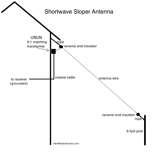
1. Long Wire Antenna

Or,

A simple 10-20 meter wire can work extremely well for shortwave listening for SW band of the radio.

Example setup:

Radio → 9:1 Unun → 15m wire antenna

Height recommendation:

3 – 10 meters above ground

2. Magnetic Loop Antennas

Magnetic loops are excellent for urban environments where electrical noise is high.

Popular models include:

• MLA-30 Active Loop
• YouLoop Passive Loop
• Airspy HF Loop

Advantages:

• Low noise pickup
• Compact size
• Works well indoors

3. Active Loop Antennas

Active loops include a built-in amplifier and can receive weak signals effectively.

However placement is critical to avoid amplifying noise. 

3. Reduce Electrical Noise

Modern homes contain many devices that generate RF interference:

• LED lighting
• Switching power supplies
• Wi-Fi routers
• Computers
• Phone chargers
• Solar power inverters

These devices raise the noise floor and mask weak signals.

Practical Noise Reduction Tips

• Move the antenna away from buildings
• Operate the radio using battery power
• Install ferrite chokes on cables
• Turn off nearby switching power supplies

4. Gain Settings on Malahit SDR

Correct gain configuration is essential. Many beginners set gain too high, which causes overload and distortion. The Malahit SDR offers extensive gain and DSP control, allowing the user to optimize reception.

Key parameters include:

• RF Gain

• Preamp

• Attenuator

• AGC

• Noise Reduction

• Bandwidth filters

The receiver allows RF gain adjustment from 0 to 59 levels

Many beginners make this mistake, Maximum gain = best reception.This is incorrect.

Too much gain causes:

• Overload

• Intermodulation distortion

• Increased noise floor

Recommended Baseline Settings

Parameter	Recommended Value
RF Gain	20 – 30
Preamp	OFF
AGC	Slow
Noise Reduction	Low
Filter Bandwidth	3-5 kHz

Increase gain slowly while watching the waterfall display, adjust gradually depending on signal strength.

When to enable Preamp

Enable the preamp only when:

• Using small antennas

• Listening to weak signals

• Operating indoors

But avoid preamp if strong broadcast stations are nearby.

When to use Attenuation

If the waterfall shows:

• Strong wide signals

• Distorted audio

• Multiple ghost signals

Then activate 10-20 dB attenuatio

5. DSP Filtering

The Malahit SDR includes powerful digital signal processing tools.The Malahit SDR includes powerful DSP features:

• Adaptive Noise Reduction

• Noise Blankers

• Variable Bandwidth Filters

• Auto Notch Filtering

These tools dramatically improve weak signal readability.

Recommended bandwidth settings:

Mode	Bandwidth
AM Broadcast	5-8 kHz
Shortwave AM	3-5 kHz
SSB	2.2-2.8 kHz
CW	300-500 Hz

Noise reduction can greatly improve weak signals. Adaptive noise reduction helps suppress background noise and improves intelligibility

6. Example Setup

Receiver Malahit DSP SDR V3

Antenna 15m long wire

Frequency 9.585 MHz

Mode AM

Recommended settings:

RF Gain: 25
Preamp: OFF
AGC: Slow
Noise Reduction: Level 10
Bandwidth: 4kHz

Expected improvement:

• Lower noise floor

• Clearer audio

• Stable signal

7. Advanced Tips for Serious DX Listening

Use a balun or unun

Improves impedance matching.

Example: 9:1 unun for long wire

Use coax feedline

Reduces noise pickup. 

Example: RG-58 or RG-174 cable

Install antenna outdoors

Outdoor antennas outperform indoor antennas by a large margin.

Monitor propagation

Websites such as:

• Solar flux reports

• DX cluster networks

• Shortwave schedules

help predict good listening times.

Conclusion

The Malahit DSP SDR V3 is capable of excellent performance when properly configured.

The three most important improvements are:

• Better antenna placement
• Lower electrical noise
• Correct gain settings

With these techniques the radio can receive shortwave signals from across the globe.

References

 

• Malahit DSP User Manual
  https://fms.komkon.org/Malahit/Malahit-Manual.pdf

• RTL-SDR Blog – Improving Malachite DSP Sensitivity
  https://www.rtl-sdr.com/improving-sensitivity-on-the-malachite-dsp-via-usb-grounding/

• N9EWO Malahit DSP Review
  https://www.qsl.net/n9ewo/malahit.html

• Malahit SDR Receiver Feature Overview
  https://manuals.plus